Analysis of 10x genomics scRNA-seq data using sincei#

The data used here is produced in our 10x genomics multiome tutorial.

We will use the BAM files, barcodes and peaks.bed file obtained from the cellranger-arc workflow. Alternatively, the BAM file (tagged with cell barcodes) and peaks.bed can be obtained from a custom mapping/peak calling workflow, and the list of filtered cell barcodes can be obtained using sincei (see the parent tutorial for explanation).

Define common bash variables:

cd 10x_multiome_testdata
# create dir
mkdir sincei_output/rna

Additionally, we will need a blacklist file to filter out reads aligned to known problematic regions of the human genome. This file and blacklists for other genome assemblies can be downloaded from the Boyle lab ENCODE blacklist repository.

wget -O hg38-blacklist.v2.bed.gz https://github.com/Boyle-Lab/Blacklist/blob/master/lists/hg38-blacklist.v2.bed.gz

2. Quality control - I (read-level)#

In order to identify high quality cells for our analysis, we can use the read-level quality statistics from scFilterStats. Low quality cells in this data can be identified using several criteria, such as:

high number of PCR duplicates (filtered using --duplicateFilter)
high fraction of reads aligned to blacklisted regions (filtered using --blackListFileName)
high fraction of reads with poor mapping quality (filtered using --minMappingQuality)
vey high/low GC content of the aligned reads, indicating the reads were mostly aligned to low-complexity regions (filtered using --GCcontentFilter)
high level of secondary/supplementary alignments (filtered using --samFlagExclude/Include)

for rep in rep1 rep2
do
   bamfile=cellranger_output_${rep}_gex_possorted_bam.bam
   barcodes=sincei_output/rna/rna_barcodes_filtered_${rep}.txt # from sincei or cellranger output
   blacklist=hg38-blacklist.v2.bed

   scFilterStats -p 8 \
      --GCcontentFilter '0.2,0.8' \
      --minMappingQuality 10 \
      --samFlagExclude 256 \
      --samFlagExclude 2048 \
      --blackListFileName ${blacklist} \
      --barcodes ${barcodes} \
      --cellTag CB \
      --label rna_${rep} \
      -o sincei_output/rna/scFilterStats_output_${rep}.tsv \
      -b ${bamfile}
done

scFilterStats summarizes these outputs as a table, which can then be visualized using the MultiQC tool, to select appropriate list of cells to include for counting.

multiqc sincei_output/rna/ # results in multiqc_report.html

3. Signal aggregation (counting reads)#

Below we use sincei to aggregate signal from single-cells. For gene expression data, we aggregate the signal from reads mapping to genes. For this we can use a GTF file containing gene annotations.

If needed, we can use the same parameters as in scFilterStats to count only high quality reads from our whitelist of barcodes.

## Download the GTF file
curl -o sincei_output/hg38.gtf.gz http://hgdownload.soe.ucsc.edu/goldenPath/hg38/bigZips/genes/hg38.refGene.gtf.gz
gunzip sincei_output/hg38.gtf.gz

# count reads on the GTF file
for rep in rep1 rep2
do
   bamfile=cellranger_output_${rep}_gex_possorted_bam.bam
   barcodes=sincei_output/rna/rna_barcodes_filtered_${rep}.txt # from sincei or cellranger output
   genes_gtf=hg38.gtf

   scCountReads features -p 8 \
      --BED ${genes_gtf} \
      --minMappingQuality 10 \
      --samFlagExclude 256 \
      --samFlagExclude 2048  \
      --blackListFileName ${blacklist} \
      --barcodes ${barcodes} \
      --cellTag CB \
      -o sincei_output/rna/scCounts_rna_genes_${rep} \
      --label rna_${rep} \
      -b ${bamfile}
done
# Number of bins found: 74538

4. Quality control - II (count-level)#

After counting, it is recommended to perform QC on these counts, in order to filter regions and cells that have low counts, or have low enrichment of counts. Even though we already performed read-level QC before, the counts distribution on our specified regions (bins/genes/peaks) could be different from the whole-genome stats.

We can run scCountQC on the count data to get various statistics at region and cell level. Running this tool with the --describe flag lists the metrics that can be used to filter cells/regions.

# list the metrics we can use to filter cells/regions
for rep in rep1 rep2
do
   scCountQC -i sincei_output/rna/scCounts_rna_genes_${rep}.h5ad --describe
done

The tool scCountQC can be used for count-level QC and filtering of count data. With the --outMetrics option, the tool outputs the count statistics at region and cell level (labelled as <prefix>.regions.tsv and <prefix>.cells.tsv). Just like scFilterStats, these outputs can then be visualized using the MultiQC tool, to select appropriate metrics to filter out the unwanted cells/regions.

# export the single-cell level metrics
for rep in rep1 rep2
do
   scCountQC -i sincei_output/rna/scCounts_rna_genes_${rep}.h5ad \
   -om sincei_output/rna/countqc_rna_genes_${rep}
done

# visualize output using multiQC
multiqc sincei_output/rna/ # see results in multiqc_report.html

In this example, we detect >74500 genes in >13.7K cells here.

Below, we perform some basic filtering using scCountQC. We exclude the cells with <500 and >10000 detected peaks (--filterRegionArgs). We also exclude peaks detected in too few cells (<100) or in >90% of cells (--filterCellArgs).

for rep in rep1 rep2
do
   scCountQC -i sincei_output/rna/scCounts_rna_genes_${rep}.h5ad \
      -o sincei_output/rna/scCounts_rna_genes_filtered_${rep}.h5ad \
      -om sincei_output/rna/scCounts_rna_genes_${rep} \
      --filterRegionArgs "n_cells_by_counts: 100, 1500" \
      --filterCellArgs "n_genes_by_counts: 500, 15000"
done

## rep 1
# Applying filters
# Cells post-filtering: 1092
# Features post-filtering: 32888
## rep 2
# Applying filters
# Cells post-filtering: 1038
# Features post-filtering: 32793

5. Combine counts for the 2 replicates#

While it is recommended to perform count QC separately for each replicate, the counts can now be combined into one file for more convenient for downstream analysis. We provide a tool scCombineCounts, which can concatenate counts for cells based on common features (in multi-sample mode). It can also be used to concatenate different modalities based on a common set of cells (in multi-modal mode).

Concatenating the filtered cells for the 2 replicates results in a total of ~12K cells.

scCombineCounts \
   -i sincei_output/rna/scCounts_rna_genes_filtered_rep1.h5ad \
   sincei_output/rna/scCounts_rna_genes_filtered_rep2.h5ad \
   -o sincei_output/rna/scCounts_rna_genes_filtered.merged.h5ad \
   --method multi-sample \
   --labels rep1 rep2
# Combined cells: 2130
# Combined features: 31976

5. Dimensionality reduction and clustering#

Finally, we will apply glmPCA to this data, assuming the data follows a poisson distribution (which is appropritate for scRNA-seq count data), we will reduce the dimensionality of the data to 20 principal components (the default), followed by a graph-based (Leiden) clustering of the output.

scClusterCells -i sincei_output/rna/scCounts_rna_genes_filtered.merged.h5ad \
   -m glmPCA \
   -gf poisson \
   --clusterResolution 0.8 \
   -op sincei_output/rna/scClusterCells_UMAP.png \
   -o sincei_output/rna/scCounts_rna_genes_clustered.h5ad

# Coherence Score:  Coherence Score:  -0.9893882070519782
# also produces the tsv file "sincei_output/rna/scClusterCells_UMAP.tsv"

(optional) Confirmation of clustering using metadata#

Below, we load this data in R and compare it to the cell metadata provided with our files to verify that our clustering separates celltypes in a biologically meaningful way.

We can color our UMAP output from scClusterCells with the cell-type information from Persad et. al. (2023), that we provide on figshare

Clustering validation (click for Python code)

import scanpy as sc
import pandas as pd
import matplotlib.pyplot as plt

# load metadata and anndata
rna_metadata = pd.read_csv('metadata_cd34_rna.csv', header=0, index_col=0)

rna_adata = sc.read_h5ad('sincei_output/rna/scCounts_rna_genes_clustered.h5ad')
rna_adata.obs_names = rna_adata.obs_names.str.replace('rep1_|rep2_', '', regex=True)

rna_adata.obs = rna_adata.obs.merge(rna_metadata['celltype'], left_index=True, right_index=True, how='left')

# make plots
colors = plt.colormaps['Paired'].colors
colors_dict = {
   # leiden clusters
   '0': colors[1],
   '1': colors[0],
   '2': colors[5],
   '3': colors[3],
   '4': colors[2],
   '5': colors[6],
   '6': colors[4],
   '7': colors[7],
   '8': colors[8],
   # published cell types
   'CLP': colors[4],
   'Ery': colors[6],
   'HMP': colors[5],
   'HSC': colors[1],
   'MEP': colors[2],
   'Mono': colors[0],
   'cDC': colors[3],
   'pDC': colors[7],
   }

sc.pl.umap(
   rna_adata,
   color=['leiden', 'celltype'],
   palette=colors_dict,
   title=['sincei Clusters (glmPCA + Leiden)', 'Published Cell Types'],
   legend_loc='on data',
   legend_fontsize=14,
   frameon=False,
   size=60,
   )

for ax in plt.gcf().axes:
   ax.title.set_size(fontsize=16)

plt.savefig("sincei_output/rna/UMAP_compared_withOrig.png", dpi=300, bbox_inches="tight")

Clustering validation (click for R code)

library(dplyr)
library(magrittr)
library(ggplot2)
library(patchwork)

umap <- read.delim("sincei_output/rna/scClusterCells_UMAP.tsv")
meta <- read.csv("metadata_cd34_rna.csv", row.names = 1)
umap$celltype <- meta[gsub("rep1_|rep2_", "", umap$Cell_ID), "celltype"]


# keep only cells with published labels
umap %<>% filter(!is.na(celltype))

# make plots
df_center <- group_by(umap, cluster) %>%
summarise(UMAP1 = mean(UMAP1),  UMAP2 = mean(UMAP2))
df_center2 <- group_by(umap, celltype) %>%
summarise(UMAP1 = mean(UMAP1), UMAP2 = mean(UMAP2))

# colors for metadata (8 celltypes)
col_pallette <- RColorBrewer::brewer.pal(8, "Paired")
names(col_pallette) <- unique(umap$celltype) # grey is for NA

# colors for sincei UMAP (9 clusters)
colors_cluster <- RColorBrewer::brewer.pal(9, "Paired")
names(colors_cluster) <- unique(umap$cluster)

p1 <- umap %>% ggplot(., aes(UMAP1, UMAP2, color=factor(cluster), label=cluster)) +
geom_point() +
geom_label(data = df_center, aes(UMAP1, UMAP2), fill = "white") +
scale_color_manual(values = colors_cluster) +
theme_void(base_size = 12) + theme(legend.position = "none") +
ggtitle("sincei Clusters (glmPCA + Leiden)")

p2 <- umap %>% filter(!is.na(celltype)) %>% ggplot(., aes(UMAP1, UMAP2,
color=factor(celltype), label=celltype)) +
geom_point() +
geom_label(data = df_center2, aes(UMAP1, UMAP2), fill = "white") +
scale_color_manual(values = col_pallette) + labs(color="Cluster") +
theme_void(base_size = 12) + theme(legend.position = "none") +
ggtitle("Published Cell Types")

pl <- p1 + p2
ggsave(plot=pl, "sincei_output/rna/UMAP_compared_withOrig.png",
dpi=300, width = 11, height = 6)

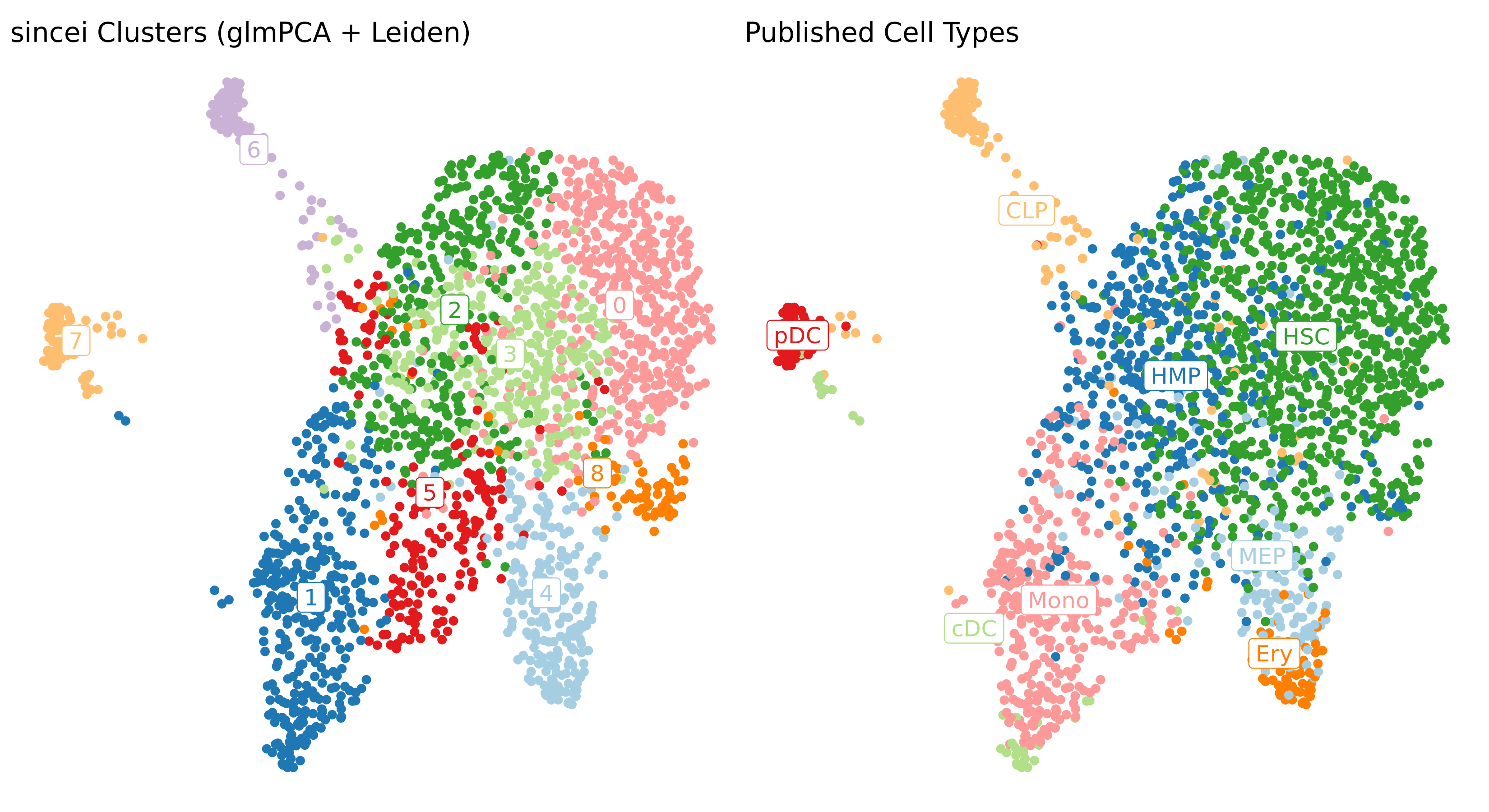
../../_images/UMAP_compared_withOrig_10xRNA.png

The figure above shows that we can easily replicate the expected cell-type results from the scRNA-seq data using sincei. However there are some interesting differences, especially, a separation of the CLP cluster into 2 clusters, where one of these clusters is similar to the annotated pDC.

This was done using basic pre-processing steps, therefore the results should only improve with better cell/region filtering and optimizing the analysis parameters.

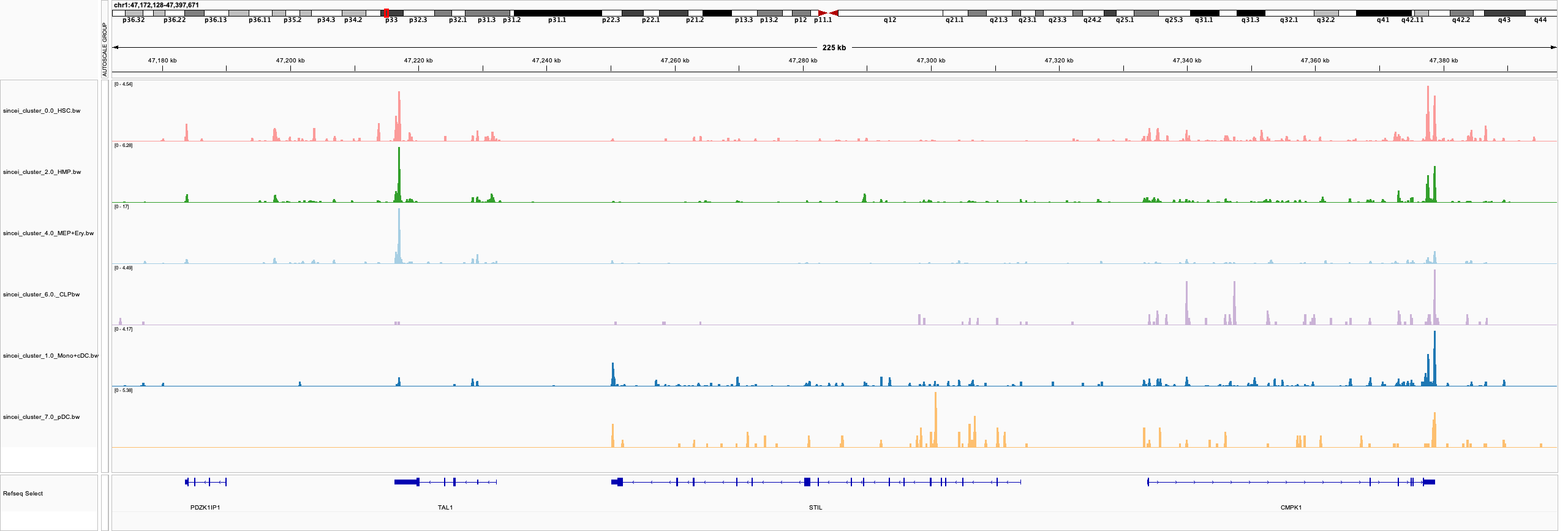
6. Creating bigwigs and visualizing signal on IGV#

For further exploration of data, it can be useful to create pseudo-bulk coverage files (bigwigs) that aggregate the signal across cells in our each of our clusters. The tool scBulkCoverage takes the clustering information .tsv file produced by scClusterCells, along with the corresponding BAM files, and aggregates the signal to create these bigwigs.

The parameters here are same as other sincei tools that work on BAM files, except that we can output normalized bulk signal (specified using --normalizeUsing option) . Below, we produce CPM-normalized bigwigs at 100bp resolution.

scBulkCoverage -p 8 \
   --cellTag CB \
   --normalizeUsing CPM \
   --binSize 100 \
   --minMappingQuality 10 \
   --samFlagExclude 2048 \
   -b cellranger_output_rep1_gex_possorted_bam.bam \
   cellranger_output_rep2_gex_possorted_bam.bam \
   --labels rep1_rna_rep1 rep2_rna_rep2 \
   -i sincei_output/rna/scClusterCells_UMAP.tsv \
   -o sincei_output/rna/sincei_cluster
# creates 11 files with names "sincei_cluster_<X>.bw" where X is 0, 1... 10

We can now inspect these bigwigs on IGV. Looking at the region around one of the markers described in the original manuscript, TAL1, we can see that the CLPs (lymphoid) and pDCs lack its expression, while the myeloid cells and HSCs present enriched signal. The neighboring gene STIL, which is involved in cell-cycle regulation is not expressed in the highly proliferative HSC/HMP/MEP cell clusters. Overall this confirms that the signal coverage extracted from our clusters broadly reflects the biology of the underlying cell types.

Analysis of 10x genomics scRNA-seq data using sincei

Contents