GLM-PCA analysis of single-cell methylome data#
Starting from the publicly available single-cell methylation data from snmCATseq , we re-processed a subset of the data to extract methlated/unmethylated reads in small genomics bins (10kb), yielding non-Gaussian data (see tutorial on preprocessing here).
This data was stored as pickle files snmC2Tseq_eckerlab/10k_bin/processed_data_*_2024_06_13.pkl, which we will import here.
Another file named mmc5.xlsx contains metadata for celltype identification.
The data losely follows a Beta distribution, and we thus employ GLM-PCA with Beta distribution to find a lower-dimension representation.
[ ]:
import tqdm, umap
import torch
import numpy as np
import pandas as pd
import seaborn as sns
import matplotlib.pyplot as plt
from sklearn.decomposition import PCA

from sincei.GLMPCA import GLMPCA

data_type = 'HCGN'
[ ]:
import os
import warnings

warnings.filterwarnings("ignore")
os.chdir("/hpc/uu_bhardwaj/group/fsanchogomez/programs/sincei_tutorial_data")
1. Read data#
Starting from the files provided in our figshare repository, the data needs to be first processed as demonstrated in “snmCATseq_prepcessing.ipynb”. We here load the output.
In order to confirm whether glmPCA results help in identifying clusters of cells, we shall also load the celltype metadata provided in the Supplementary table 5 of the original manuscript.
[ ]:
# methylation (number of methylated covered)
df_cov = pd.read_csv(
    f"snmC2Tseq_eckerlab/processed_data_{data_type}.csv.gz",
    index_col=[0,1],
    compression='gzip'
)

X_data = df_cov.values
X_data = X_data[:, np.where(np.std(X_data,axis=0)>0.08)[0]] # Previously 0.08
Now we can open the metadata from the original manuscript. NOTE: loading it requires openpyxl. You may install it by running conda install openpyxl in your environment.
[ ]:
# Metadata from the paper
metadata_df = pd.read_excel('snmC2Tseq_eckerlab/mmc5.xlsx', sheet_name=1, header=1)

# Structure metadata
metadata_df['sample_idx'] = metadata_df['Sample'].apply(lambda x: '_'.join(x.split('_')[1:11]))
metadata_df = metadata_df.set_index('sample_idx')

X_data_index = ['_'.join(e.split('/')[-1].split('.')[0].split('_')[3:13]) for e in  df_cov.loc[data_type].index]
cell_labels = metadata_df.loc[X_data_index]
2. GLM-PCA#
To aid in this analysis, we provide two Beta families within the glmPCA framework: Beta and SigmoidBeta.
SigmoidBeta employs logit-transformed saturated parameters, which removes all optimisation constraints and is therefore much more stable.
Several hyper-parameters are hard-coded, but do not vastly influence the analysis. The only hyper-parameter which can fundamentally change the results is the learning rate. 2.5 is a good choice for sigmoid_beta, but this needs to be changed for other distributions.
[ ]:
eps = 1e-5
n_pc = 20
family = 'sigmoid_beta'

clf = GLMPCA(
    n_pc=n_pc,
    family=family,
    n_jobs=5,
    max_iter=500,
    learning_rate=10.,
)
Beta distribution not initialized yet
[ ]:
# Imputes zeros with mean
X_glm_data = X_data.copy()
for idx in tqdm.tqdm(range(X_data.shape[1])):
    non_zero_mean = X_glm_data[X_glm_data[:,idx] != 0,idx].mean()
    X_glm_data[X_glm_data[:,idx] == 0,idx] = non_zero_mean

clf.fit(torch.Tensor(X_glm_data))
100%|████████████████████████████████████████████████████████████████████████████████████████████████████████████████████████████████████████████████████████████████████████████████████████████████████████████████████████████| 9979/9979 [00:00<00:00, 28407.52it/s]
100%|█████████████████████████████████████████████████████████████████████████████████████████████████████████████████████████████████████████████████████████████████████████████████████████████████████████████████████████████| 9979/9979 [00:03<00:00, 2497.02it/s]
 22%|█████████████████████████████████████████████████▋                                                                                                                                                                                | 22/100 [00:11<00:39,  2.00it/s]
CONVERGENCE AFTER 22 ITERATIONS
LEARNING RATE: 10.0
7%|████████████████▋ | 37/500 [00:12<02:38, 2.92it/s]
        RESTART BECAUSE INF/NAN FOUND
LEARNING RATE: 5.0
100%|█████████████████████████████████████████████████████████████████████████████████████████████████████████████████████████████████████████████████████████████████████████████████████████████████████████████████████████████████| 500/500 [03:02<00:00,  2.74it/s]
  7%|████████████████▋                                                                                                                                                                                                                 | 37/500 [03:21<42:01,  5.45s/it]
True
[ ]:
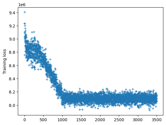
# The loss curve must converge (reach a plateau)
plt.plot(np.array(clf.loadings_learning_scores_).T, '+')
plt.ylabel('Training loss')
Text(0, 0.5, 'Training loss')
[ ]:
X_project = clf.transform(torch.Tensor(X_glm_data))
22%|█████████████████████████████████████████████████▋ | 22/100 [00:11<00:39, 2.00it/s]
CONVERGENCE AFTER 22 ITERATIONS
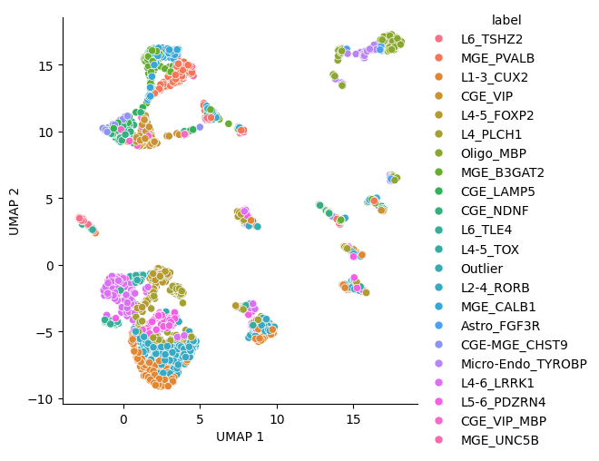
UMAP on GLM-PCA components#
[ ]:
_umap_params = {'n_neighbors':15, 'min_dist': 0.3, 'n_epochs': 1000}

metric = 'cosine'

_umap_clf = umap.UMAP(metric=metric, verbose=True, **_umap_params)
umap_embeddings = pd.DataFrame(
    _umap_clf.fit_transform(X_project.detach().numpy()),
    columns=['UMAP 1', 'UMAP 2']
).reset_index()
umap_embeddings['label'] = cell_labels['snmC2T-seq Baseline Cluster'].values

g = sns.relplot(data=umap_embeddings, x='UMAP 1', y='UMAP 2',hue='label')
figure_name = f"UMAP_glm_pca_{n_pc}_metric_{metric}_{family}"
UMAP(angular_rp_forest=True, metric='cosine', min_dist=0.3, n_epochs=1000, verbose=True)
Wed Dec 17 13:06:05 2025 Construct fuzzy simplicial set
Wed Dec 17 13:06:07 2025 Finding Nearest Neighbors
Wed Dec 17 13:06:12 2025 Finished Nearest Neighbor Search
Wed Dec 17 13:06:14 2025 Construct embedding
        completed  0  /  1000 epochs
        completed  100  /  1000 epochs
        completed  200  /  1000 epochs
        completed  300  /  1000 epochs
        completed  400  /  1000 epochs
        completed  500  /  1000 epochs
        completed  600  /  1000 epochs
        completed  700  /  1000 epochs
        completed  800  /  1000 epochs
        completed  900  /  1000 epochs
Wed Dec 17 13:06:18 2025 Finished embedding
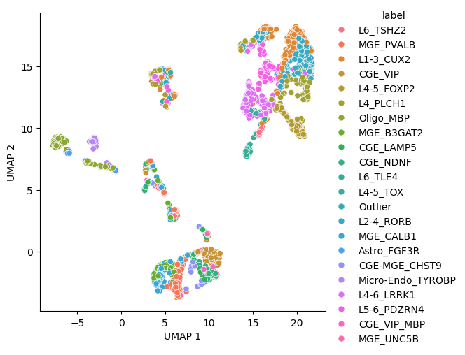
3. Compare to standard PCA.#
[ ]:
pca_clf = PCA(n_pc).fit(X_data)
X_pca = pca_clf.transform(X_data)
UMAP on standard PCA components#
[ ]:
_umap_params = {'n_neighbors':15, 'min_dist': 0.3, 'n_epochs': 1000}

metric = 'cosine'
_umap_clf = umap.UMAP(metric=metric, verbose=True, **_umap_params)
umap_embeddings = pd.DataFrame(
    _umap_clf.fit_transform(X_pca),
    columns=['UMAP 1', 'UMAP 2']
).reset_index()
umap_embeddings['label'] = cell_labels['snmC2T-seq Baseline Cluster'].values

g = sns.relplot(data=umap_embeddings, x='UMAP 1', y='UMAP 2',hue='label')
UMAP(angular_rp_forest=True, metric='cosine', min_dist=0.3, n_epochs=1000, verbose=True)
Wed Dec 17 13:06:23 2025 Construct fuzzy simplicial set
Wed Dec 17 13:06:25 2025 Finding Nearest Neighbors
Wed Dec 17 13:06:25 2025 Finished Nearest Neighbor Search
Wed Dec 17 13:06:25 2025 Construct embedding
        completed  0  /  1000 epochs
        completed  100  /  1000 epochs
        completed  200  /  1000 epochs
        completed  300  /  1000 epochs
        completed  400  /  1000 epochs
        completed  500  /  1000 epochs
        completed  600  /  1000 epochs
        completed  700  /  1000 epochs
        completed  800  /  1000 epochs
        completed  900  /  1000 epochs
Wed Dec 17 13:06:28 2025 Finished embedding
4. Compare directions found by GLM-PCA and standard PCA#
We can compare the results we obtained using a Beta GLM-PCA with standard PCA by calculating the cosine similarity between each component.
[ ]:
M = clf.saturated_loadings_.detach().numpy().T.dot(pca_clf.components_.T)
sns.heatmap(M, cmap='seismic_r', center=0, vmax=1, vmin=-1)
plt.ylabel('Beta GLM-PCA', fontsize=16)
plt.xlabel('Standard PCA', fontsize=16)
plt.xticks(fontsize=10, rotation=0)
plt.yticks(fontsize=10, rotation=0)
plt.title('Cosine similarity', fontsize=18)

plt.tight_layout()
plt.show()
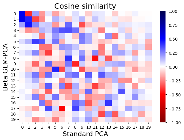
We observe that the first two components are closely related, a cosine similarity close to 1 indicates that they “point in the same direction” in the high-dimensional feature space. A few other components have high cosine similarities, but most are not highly related.